Fundy MVP Transect August 3rd 2006

Fundy Oceanographic Transect
CCGS Frederick G. Creed
August 3rd 2006

John E. Hughes Clarke
Ocean Mapping Group
University of New Brunswick

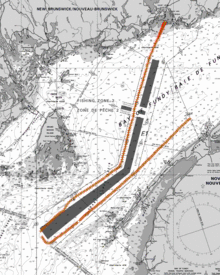
A pair of oceanographic transects were obtained by JEHC on the 3rd of August 2006 onboard the CCGS Frederick G. Creed. The data were obtained using a BOT-MVP-100 outfitted with an AML Sv,T & Z probe. The MVP was set to cycle automatically, achieving a depth of ~ 80m on average at 12 knots with an inter-dip spacing of ~ 500m.

Outbound profile (Saint John Harbour to Gulf of Maine) - dips 005 - 173

Inbound profile (Gulf of Maine to Approaches to Digby Basin) dips 174 - 295

By inverting the Chen and Millero relationship, one can estimate the salinity from the temperature, sound speed and depth of the sensor output. Using the temperature, depth and derived salinity, the density can in-turn be derived using the UNESCO formulae.

LABORATORY EXERCISE - GGE5013 - Autumn 2006

Data Manipulation
- Outward bound dips only (005-173)

download the data
plot up the locations (see if you can find a suitable cartographic backdrop image)
calculate the time and distance (and speed) between dips and make a plot to see what penetration an MVP-100 can achieve as function of speed and depth.
plot the bottom depth along the profiles by distance (can be found in each ascii file)
plot up the temperature and sound speed profiles of the outward bound profiles - show the 0-120m depth range
using the T, Vp and Z, try to estimate the Salinity for each sample.
draw a distance - profile of the near surface (1-3m) temperature, salinity and sound speed along the transect.
using the T, Z and derived Salinity, try to estimate the Density for each sample.
plot up the salinity and density profiles of the outward bound profile - show the 0-120m depth range
make a display of the cross section profiles of Vp, T, S and density by distance along the outward profile
Calculate and plot a section of the Brunt Vaisala (buoyancy) frequency profile for each dip.

8/20 for the above.....

To help you get going a skeleton C program is available here.
This should speed up the manipulation of the raw data to make useful plots etc...

Data Interpretation

Significance to the Oceanographic Environment

Explain the main oceanographic features visible in the profile.

3/20

Try to obvtain a SST image of the region. Go to :
http://wavy.umeoce.maine.edu/frames.html

Try to find cloud free images as close in time to the profile observed. You may have to go forward or back a few days.

Try to plot the profile across the image (can you register the image?).
Can you see any resemblence between the SST image and the surface temperature plot that you made .
Can you see any differences?
How variable is the SST inthat area from image to image and from day to day ?
Would the profile have been similar if the section had been made further to the north or south?

3/20

Consequences for Hydrographic Survey

Controls on Sound Speed Structure:

Compare and contrast the relative importance of temperature versus salinity in influencing the sound speed cross-section.
3/20

Estimating the Sensitivity of the refracted ray path to water column structure:

Pick 5 end-member Vp profiles that are representative of the main watermasses seen.

Pick one and do a ray trace for a beam (starting at a depth of 3m) with the following launch angles of 0, 30 50 65 & 70 degrees until you reach a depth of 75m.
Extract the TWTT to reach that depth for that profile for each of the angles (and record the across-track distance achieved).

For each of the other 4 profiles, using the same TWTT, see what depth and across-track distance you would achieve.

What is the range of depth and across-track errors ?
What does this mean in terms of IHO acceptance ?

3/20

DATA

Ascii Listing of Geographic Coordinates of each dip HERE

gzipped tarfile of each MVP dip for outbound track HERE

gzipped tarfile of each MVP dip inbound track HERE

page generated by JEHC on September 25th 2006